
Study of Discretization Techniques in the context of Distributed Genetic Classifiers
Authors
- L. Ignacio Lopez
- Juan M. Bardallo
- Miguel A. De Vega
- Antonio Peregrin
- Paper abstract
-
Discretized data sets
5fcv partitions for the 42 data sets used in the paper, all of them discretized with all the methods presented in the paper.
-
Discretized data sets with SMOTE
5fcv partitions for the 42 data sets used in the paper, all of them discretized with all the methods presented in the paper and balanced using SMOTE procedure.
-
Data sets indexes
Results of the indexes presented in the paper for each of the data sets.
-
Algorithm results
Results obtained for Distributed and Non-distributed algorithms with all the discretizers used in the paper
-
Study of the Discretization Techniques and Non-Distributed Classifiers
Brief description of the results obtained for a set of Non-distributed classifiers with all the discretizers used in the paper
-
Discretizer results
Results obtained for all the discretizers with distributed classifiers used in the paper and a set of Non-distributed classifiers.
1. Abstract
Since most real-world applications of classification learning involve continuous valued attributes, the discretization process is known to be one of the most important pre-processing or data reduction steps. Properly addressing the discretization process is an important issue with a great impact on classification algorithm performance. In this paper, in the context of data mining and classification tasks, the interrelationships among the three elements that make up the 3-tuple [data set, discretizer, classification algorithm] are analysed. We studied the impact of the discretization process on both datasets and the classi cation task. We are especially concerned with distributed genetic algorithms and the development of a method based on data complexity measures to find the right discretizer with a previously chosen competent classifier for the problem at hand. Despite the specific and concrete results obtained in this research, from the empirical evidence we could extend the scope of no free lunch theorem to the discretization process, because with no prior information there is no better discretizer for all types of data and the use of one or another depends on the dataset complexity and the features of the classification algorithm.
2. Discretized data sets
We considered forty two data sets from UCI with different ratios between the minority and majority classes: from low imbalance to highly imbalanced datasets. Multiclass data sets were modified to obtain two-class non-balanced problems, so that the union of one or more classes became the positive class and the union of one or more of the remaining classes was labelled as the negative class. Table 1 and Table 2 summarizes, respectively, the imbalanced data and balanced data using SMOTE employed in the paper and shows, for each data set, the number of attributes (#Atts.), number of examples (#Ex.), (IR) Imbalance rate and one column for each discretizer. These tables are arranged according to the IR column, from low to high imbalance.
Table 1
| Data set | #Atts. (R/I/N) | #Ex. | IR | CADD | CAIM | ChiMerge | Chi2Merge | MDLP | ID3 | USD |
|---|---|---|---|---|---|---|---|---|---|---|
| glass1 | 9 (9/0/0) | 214 | 1.82 | |||||||
| pima | 8 (8/0/0) | 768 | 1.87 | |||||||
| glass0 | 9 (9/0/0) | 214 | 2.06 | |||||||
| yeast1 | 8 (8/0/0) | 1484 | 2.46 | |||||||
| haberman | 3 (0/3/0) | 306 | 2.78 | |||||||
| vehicle1 | 18 (0/18/0) | 846 | 2.9 | |||||||
| vehicle3 | 18 (0/18/0) | 846 | 2.99 | |||||||
| vehicle0 | 18 (0/18/0) | 846 | 3.25 | |||||||
| ecoli1 | 7 (7/0/0) | 336 | 3.36 | |||||||
| ecoli2 | 7 (7/0/0) | 336 | 5.46 | |||||||
| yeast3 | 8 (8/0/0) | 1484 | 8.1 | |||||||
| ecoli3 | 7 (7/0/0) | 336 | 8.6 | |||||||
| page-blocks0 | 10 (4/6/0) | 5472 | 8.79 | |||||||
| ecoli-0-3-4vs5 | 7 (7/0/0) | 200 | 9 | |||||||
| yeast-2vs4 | 8 (8/0/0) | 514 | 9.08 | |||||||
| ecoli-0-6-7vs3-5 | 7 (7/0/0) | 222 | 9.09 | |||||||
| ecoli-0-2-3-4vs5 | 7 (7/0/0) | 202 | 9.1 | |||||||
| yeast-0-3-5-9vs7-8 | 8 (8/0/0) | 506 | 9.12 | |||||||
| yeast-0-2-5-6vs3-7-8-9 | 8 (8/0/0) | 1004 | 9.14 | |||||||
| yeast-0-2-5-7-9vs3-6-8 | 8 (8/0/0) | 1004 | 9.14 | |||||||
| ecoli-0-4-6vs5 | 6 (6/0/0) | 203 | 9.15 | |||||||
| ecoli-0-1vs2-3-5 | 7 (7/0/0) | 244 | 9.17 | |||||||
| ecoli-0-2-6-7vs3-5 | 7 (7/0/0) | 224 | 9.18 | |||||||
| ecoli-0-3-4-6vs5 | 7 (7/0/0) | 205 | 9.25 | |||||||
| ecoli-0-3-4-7vs5-6 | 7 (7/0/0) | 257 | 9.28 | |||||||
| yeast-0-5-6-7-9vs4 | 8 (8/0/0) | 528 | 9.35 | |||||||
| vowel0 | 13 (10/3/0) | 988 | 9.98 | |||||||
| ecoli-0-1-4-7vs2-3-5-6 | 7 (7/0/0) | 336 | 10.59 | |||||||
| glass2 | 9 (9/0/0) | 214 | 11.59 | |||||||
| ecoli-0-1-4-7vs5-6 | 6 (6/0/0) | 332 | 12.28 | |||||||
| ecoli-0-1-4-6vs5 | 6 (6/0/0) | 280 | 13 | |||||||
| glass4 | 9 (9/0/0) | 214 | 15.47 | |||||||
| ecoli4 | 7 (7/0/0) | 336 | 15.8 | |||||||
| page-blocks-1-3vs4 | 10 (4/6/0) | 472 | 15.86 | |||||||
| abalone9-18 | 8 (7/0/1) | 731 | 16.4 | |||||||
| glass-0-1-6vs5 | 9 (9/0/0) | 184 | 19.44 | |||||||
| glass5 | 9 (9/0/0) | 214 | 22.78 | |||||||
| yeast-2vs8 | 8 (8/0/0) | 482 | 23.1 | |||||||
| yeast4 | 8 (8/0/0) | 1484 | 28.1 | |||||||
| yeast5 | 8 (8/0/0) | 1484 | 32.73 | |||||||
| ecoli-0-1-3-7vs2-6 | 7 (7/0/0) | 281 | 39.14 | |||||||
| yeast6 | 8 (8/0/0) | 1484 | 41.4 |
3. Discretized data sets with SMOTE
Table 2
| Data set | #Atts. (R/I/N) | #Ex. | IR | CADD | CAIM | ChiMerge | Chi2Merge | MDLP | ID3 | USD |
|---|---|---|---|---|---|---|---|---|---|---|
| glass1 | 9 (9/0/0) | 214 | 1.82 | |||||||
| pima | 8 (8/0/0) | 768 | 1.87 | |||||||
| glass0 | 9 (9/0/0) | 214 | 2.06 | |||||||
| yeast1 | 8 (8/0/0) | 1484 | 2.46 | |||||||
| haberman | 3 (0/3/0) | 306 | 2.78 | |||||||
| vehicle1 | 18 (0/18/0) | 846 | 2.9 | |||||||
| vehicle3 | 18 (0/18/0) | 846 | 2.99 | |||||||
| vehicle0 | 18 (0/18/0) | 846 | 3.25 | |||||||
| ecoli1 | 7 (7/0/0) | 336 | 3.36 | |||||||
| ecoli2 | 7 (7/0/0) | 336 | 5.46 | |||||||
| yeast3 | 8 (8/0/0) | 1484 | 8.1 | |||||||
| ecoli3 | 7 (7/0/0) | 336 | 8.6 | |||||||
| page-blocks0 | 10 (4/6/0) | 5472 | 8.79 | |||||||
| ecoli-0-3-4vs5 | 7 (7/0/0) | 200 | 9 | |||||||
| yeast-2vs4 | 8 (8/0/0) | 514 | 9.08 | |||||||
| ecoli-0-6-7vs3-5 | 7 (7/0/0) | 222 | 9.09 | |||||||
| ecoli-0-2-3-4vs5 | 7 (7/0/0) | 202 | 9.1 | |||||||
| yeast-0-3-5-9vs7-8 | 8 (8/0/0) | 506 | 9.12 | |||||||
| yeast-0-2-5-6vs3-7-8-9 | 8 (8/0/0) | 1004 | 9.14 | |||||||
| yeast-0-2-5-7-9vs3-6-8 | 8 (8/0/0) | 1004 | 9.14 | |||||||
| ecoli-0-4-6vs5 | 6 (6/0/0) | 203 | 9.15 | |||||||
| ecoli-0-1vs2-3-5 | 7 (7/0/0) | 244 | 9.17 | |||||||
| ecoli-0-2-6-7vs3-5 | 7 (7/0/0) | 224 | 9.18 | |||||||
| ecoli-0-3-4-6vs5 | 7 (7/0/0) | 205 | 9.25 | |||||||
| ecoli-0-3-4-7vs5-6 | 7 (7/0/0) | 257 | 9.28 | |||||||
| yeast-0-5-6-7-9vs4 | 8 (8/0/0) | 528 | 9.35 | |||||||
| vowel0 | 13 (10/3/0) | 988 | 9.98 | |||||||
| ecoli-0-1-4-7vs2-3-5-6 | 7 (7/0/0) | 336 | 10.59 | |||||||
| glass2 | 9 (9/0/0) | 214 | 11.59 | |||||||
| ecoli-0-1-4-7vs5-6 | 6 (6/0/0) | 332 | 12.28 | |||||||
| ecoli-0-1-4-6vs5 | 6 (6/0/0) | 280 | 13 | |||||||
| glass4 | 9 (9/0/0) | 214 | 15.47 | |||||||
| ecoli4 | 7 (7/0/0) | 336 | 15.8 | |||||||
| page-blocks-1-3vs4 | 10 (4/6/0) | 472 | 15.86 | |||||||
| abalone9-18 | 8 (7/0/1) | 731 | 16.4 | |||||||
| glass-0-1-6vs5 | 9 (9/0/0) | 184 | 19.44 | |||||||
| glass5 | 9 (9/0/0) | 214 | 22.78 | |||||||
| yeast-2vs8 | 8 (8/0/0) | 482 | 23.1 | |||||||
| yeast4 | 8 (8/0/0) | 1484 | 28.1 | |||||||
| yeast5 | 8 (8/0/0) | 1484 | 32.73 | |||||||
| ecoli-0-1-3-7vs2-6 | 7 (7/0/0) | 281 | 39.14 | |||||||
| yeast6 | 8 (8/0/0) | 1484 | 41.4 |
4. Data sets Indexes
Results of the indexes presented in the paper for each of the data sets. Each csv file contains the results obtained with the original imbalanced data set and the balanced data set using SMOTE. These results are presented for all the discretizers presented in the paper.
Results obtained in the process of discretization of the data sets used in the paper.The aim of indexes NP1, N4, N2, F4 and AP1 is to characterize the different data sets. Particularly, we compute the indexes before and after the discretization. process to measure the changes introduced by the selected discretizers for the different datasets. Each csv file presents the results with and without SMOTE, to study the influence of this recognized preprocessing step. The last column of the table presents a sumary of the mean values and standard deviation of all indexes with each discretizer for all data sets.
Table 3
| F4 | N2 | N4 | NP1 | AP1 | Indexes Means |
|---|---|---|---|---|---|
 |
|
|
|
|
|
5. Algorithms results
In the following table we provide a csv file with the results obtained for each algorithm with all the discretizers presented in the paper. We also provide a tex file and pdf file with a set of post hoc procedures. There are two sets of results corresponding to the original imbalanced data sets and after applying SMOTE.
Table 4
| Results | Results with SMOTE | |||||
|---|---|---|---|---|---|---|
| Algorithm | Results with discretizers | Post hoc procedure Results | Results with discretizers | Post hoc procedure Results | ||
| C45Rules | |
 |
 |
|
|
|
| COGIN | |
|
|
|
|
|
| EDGAR | |
|
|
|
|
|
| GAssist | |
|
|
|
|
|
| Oblique-DT | |
|
|
|
|
|
| OCEC | |
|
|
|
|
|
| REGAL | |
|
|
|
|
|
| REGAL-TC | |
|
|
|
|
|
| Ripper | |
|
|
|
|
|
| SIA | |
|
|
|
|
|
| UCS | |
|
|
|
|
|
6. Study of the Discretization Techniques and Non-Distributed Classifiers
Following, we present the outcome and the analysis of the rest of algorithms for the sake of comparison support by means of a graphical representation of accuracy versus number of rules. The objective is to check if the behavior of the discretizers is similar that in the case of distributed algorithms. Finally we presents some conclusions obtained in the ligth of the results obtained for the non-distributed classifiers presented.
| Results |
|---|
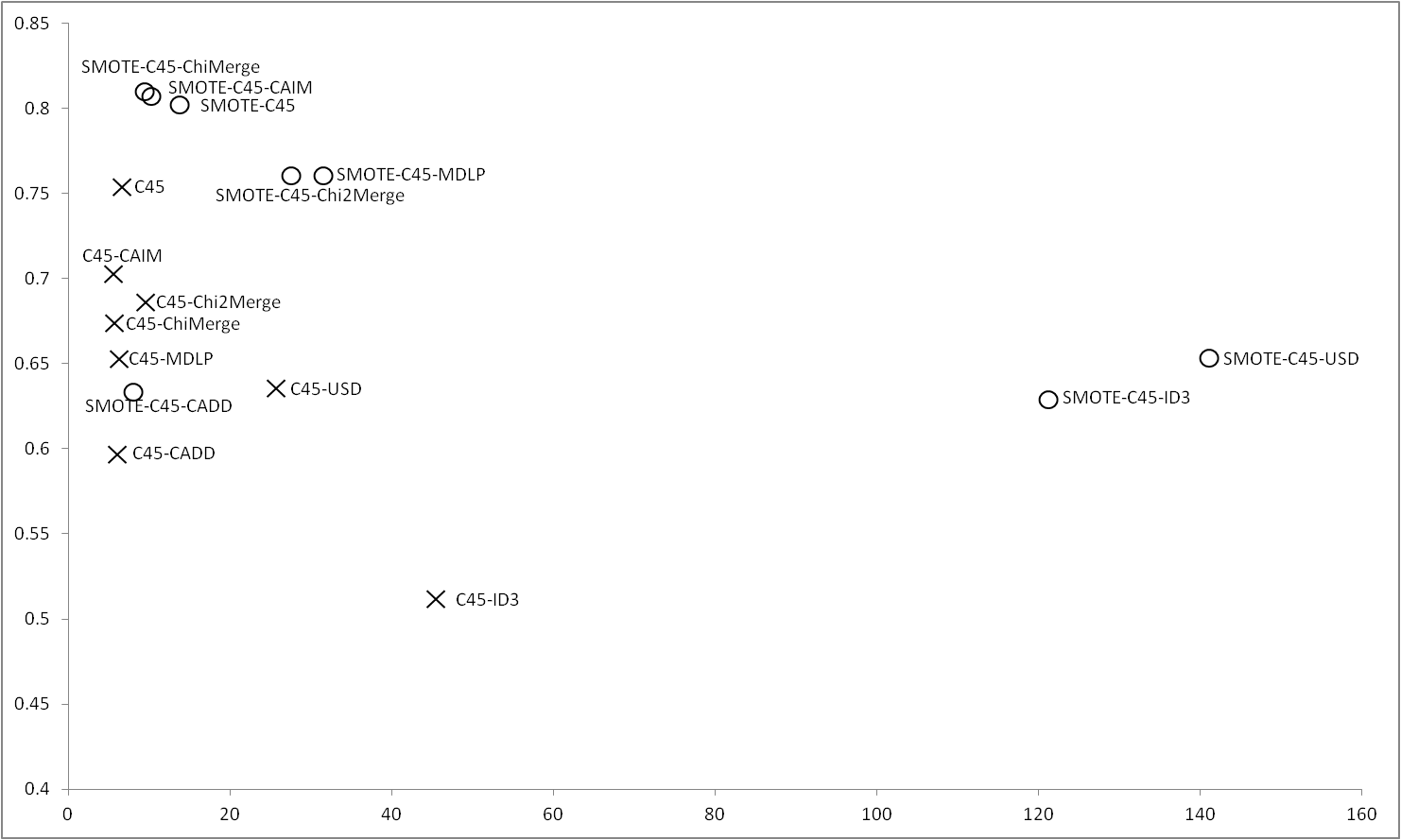
Results obtained with C45Rules |
Figure 1 shows the results obtained for C4.5 with imbalance and balanced datasets. When no SMOTE is applied C4.5 outperforms all the discretizers obtaining the best accuracy and interpretability, however, applying SMOTE, results in a great improvement in the results obtained by ChiMerge and CAIM, which obtain the best global results coupled with C4.5 without discretization step. |
Figure 1 |
 |
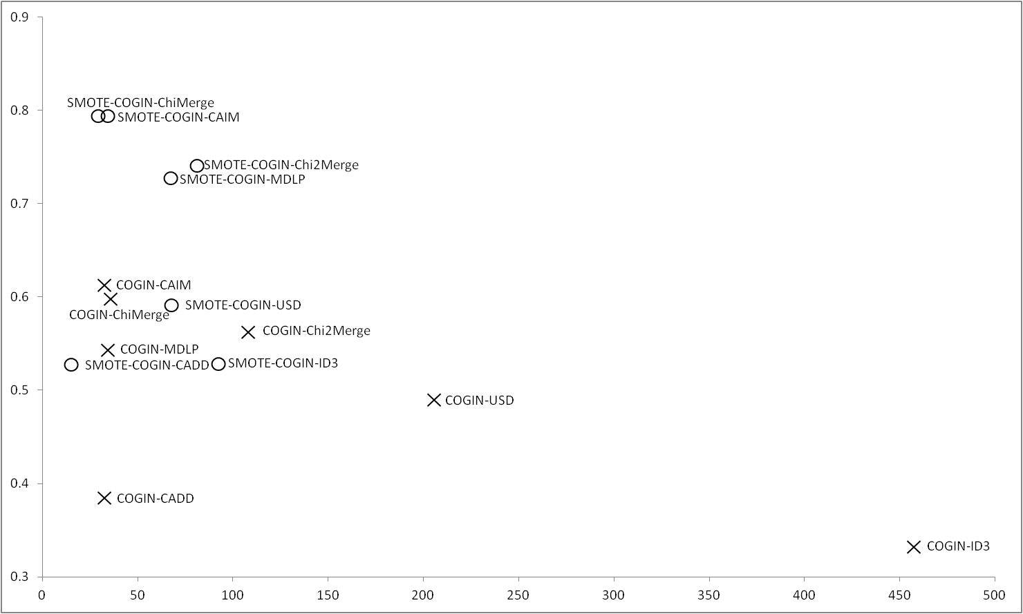
Results obtained with COGIN |
COGIN is an algorithm that does not deals with continuous values. Figure 2 shows the results obtained for all the discretizers. ChiMerge and CAIM are the discretizers whose obtain the best results using both, imbalance and balance data. In this case, there are differences between the use or not of SMOTE, using this method results an improvement in the results obtained in accuracy without an increase in the number of rules. The worst results are obtained by ID3 and CADD, obtaining the first, a high number of rules with the imbalance data. |
Figure 2 |
 |
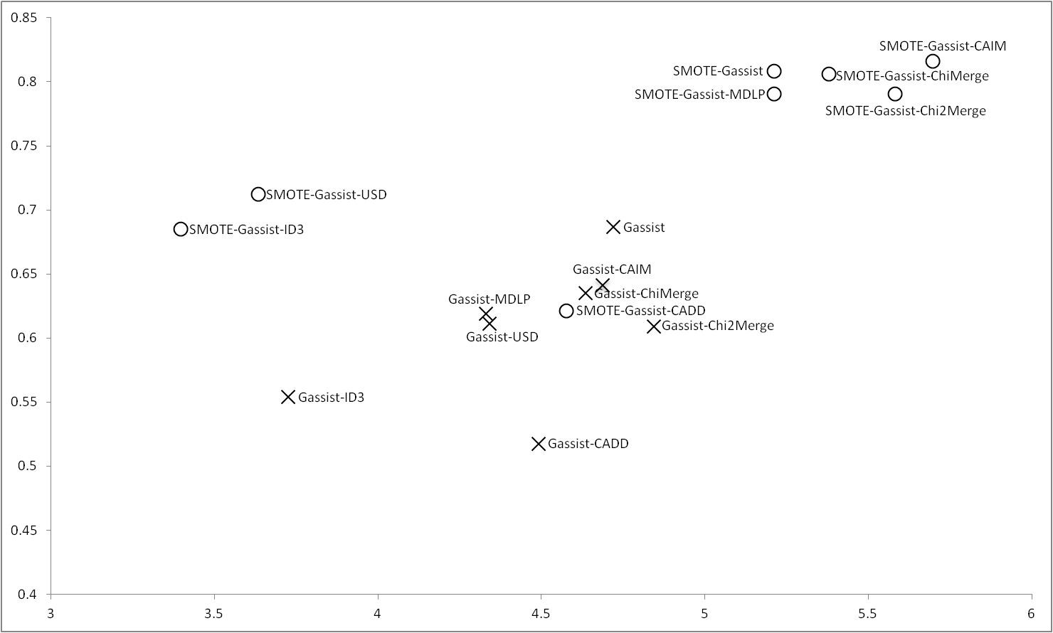
Results obtained with GAssist |
As in the case of C4.5, Gassist obtains the best results outperforming all the discretizers when it deals with raw data, however, applying SMOTE, once again ChiMerge and CAIM are able to obtain results closer to GAssist, furthermore, MDLP and Chi2Merge also obtain good results. ID3 and CADD are the worse discretizers when GAssist treats with imbalance data. USD trends to obtain similar values to ID3 when the balance process is applied. |
Figure 3 |
 |
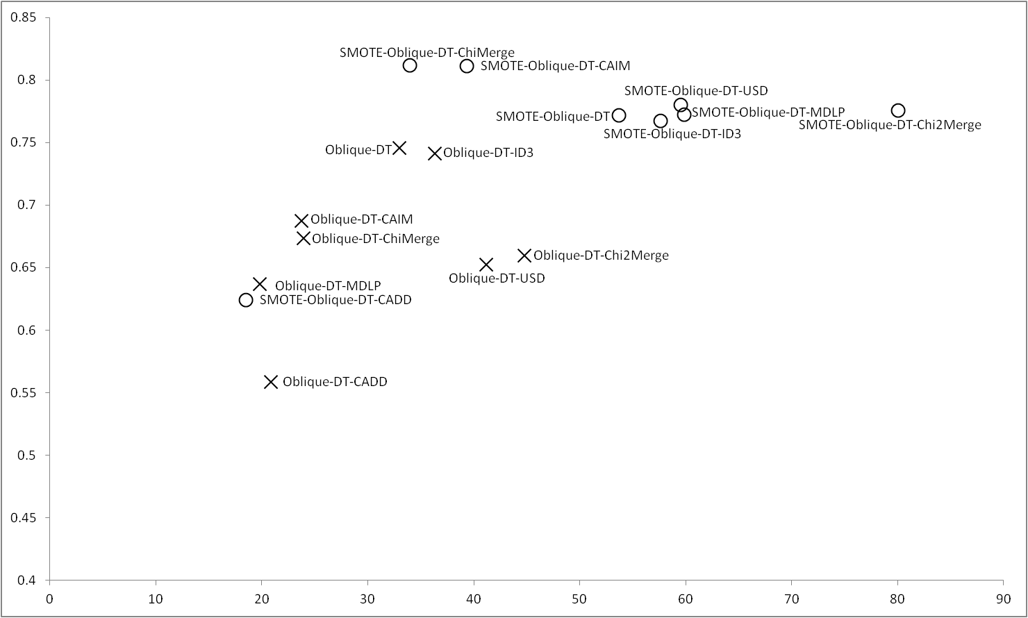
Results obtained with Oblique-DT |
Oblique-DT obtains the best results with imbalance data, only using ID3 reaches similar results, however using SMOTE are ChiMerge and CAIM whose obtain the best results, being the first which obtains the best performance with the lowest number of rules. Oblique-DT obtains similar results to USD, MDLP and ID3. Chi2Merge in this case, although obtains a good accuracy, also have a high number of rules. Regardless the balance or imbalance of the data is CADD the discretizer with the lower number of rules but at expense of obtains a poor accuracy. |
Figure 4 |
 |
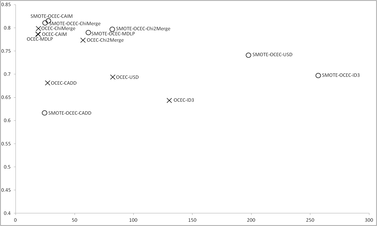
Results obtained with OCEC |
Figure 5 shows the results obtained for OCEC, unlike in other cases, OCEC does not deals with continuous values, so this results can help to choose a good discretizer to use with OCEC. With the imbalance data ChiMerge, CAIM and MDLP are the discretizers whose obtain the best results. ID3 is which obtains the worst results in this case. Applying SMOTE, ChiMerge and CAIM obtain the best results, MDLP and Chi2Merge are able to obtain good accuracy but with a greater number of rules. As in previous results, CADD worse using SMOTE, being the discretizer with the lowest performance. It can be seen that, for OCEC, the results obtained using ChiMerge and CAIM are very similar regardless the use or not of SMOTE. |
Figure 5 |
 |
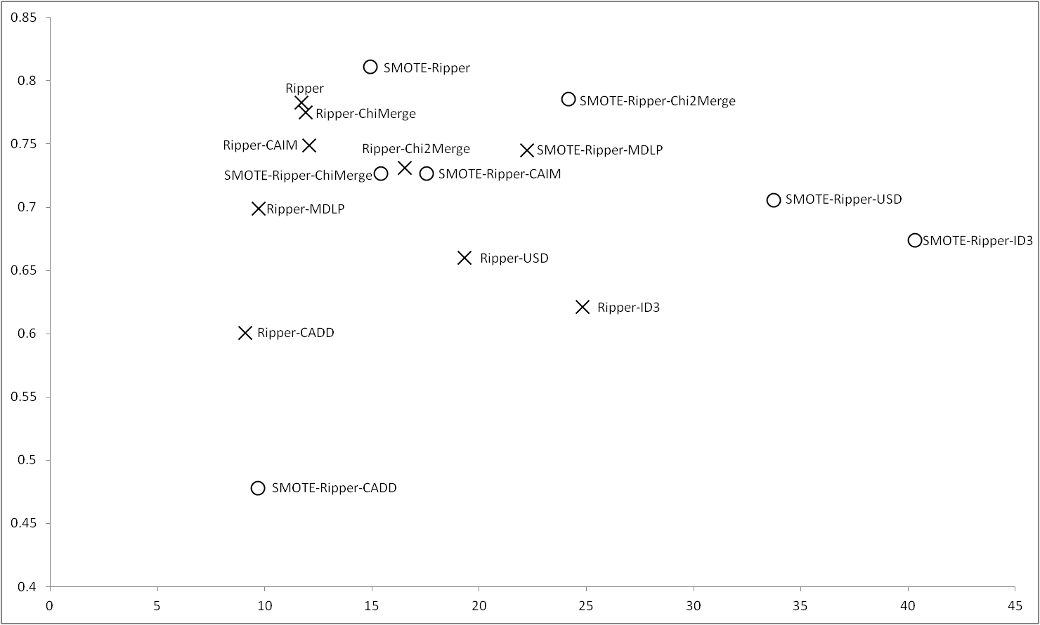
Results obtained with Ripper |
RIPPER obtains the best results regardless the use of SMOTE, in this case, unlike previous cases, when we apply SMOTE the results of the discretizers get away the results of RIPPER, which greatly increases its performance. ChiMerge and CAIM are closer treating with raw data, but with the balance of the data is Chi2Merge the discretizer which most gets closer to the results of RIPPER. In this case, we can see that CADD worse its results applying SMOTE. |
Figure 6 |
 |
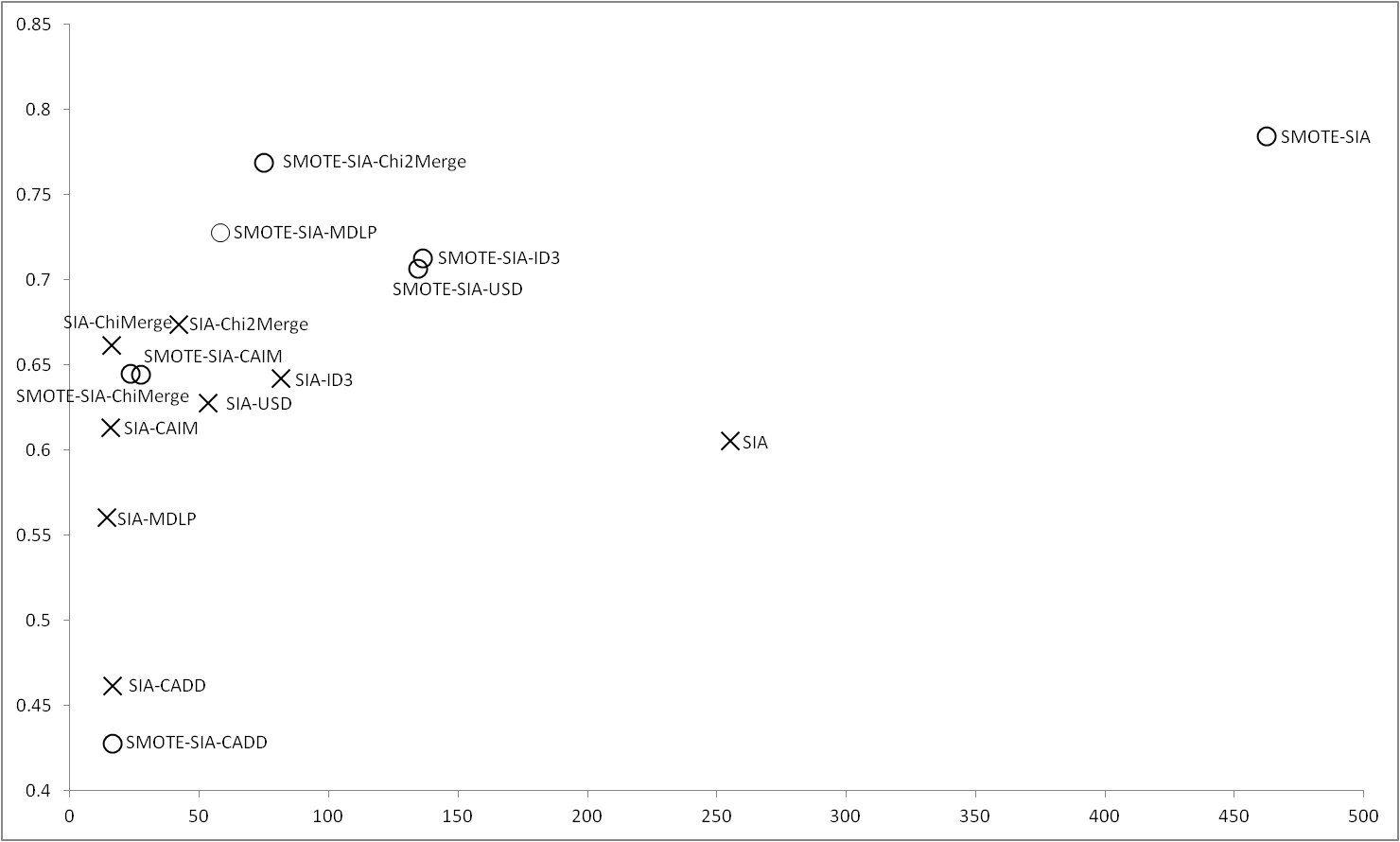
Results obtained with SIA |
In the case of SIA, using the imbalance data, the original method is outperformed when a discretizer is used, in this case, Chi2Merge and ChiMerge obtain the best results. We want to highlight that, in this case, SIA using ID3 and USD obtains a much smaller number of rules that SIA with its built-in discretizer. Applying SMOTE, although the results of SIA are the most accurate, obtains a high number of rules, however, with Chi2Merge the accuracy is closer but with a low number of rules. We also can see that MDLP is the discretizer which more improves using SMOTE, outperforming all the discretizers except Chi2Merge. |
Figure 7 |
 |
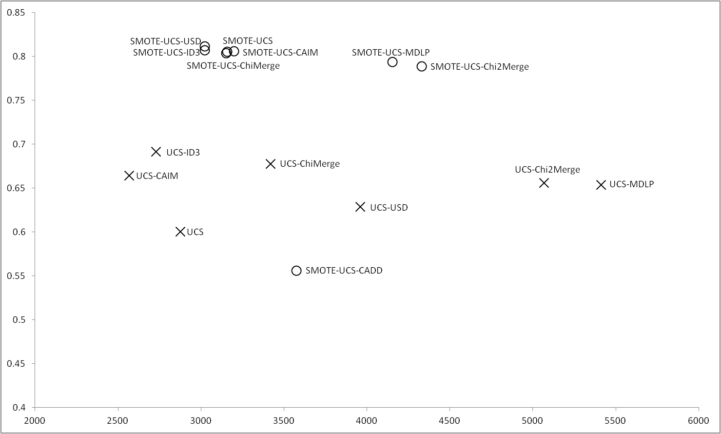
Results obtained with UCS |
Figure 8 shows the results obtained for UCS, in this case, with the imbalance datasets, the results obtained by UCS are outperformed when UCS uses a discretizer, and the best results are obtained by ID3. CAIM and ChiMerge also obtain good results. When the data are balanced using SMOTE, all the discretizers except CADD improve their results, it can be highlight that, the balance of the data makes UCS to obtain good results closely to USD discretizer, that is which obtains the best results in this case. |
Figure 8 |
 |
Discussion and concluding remarks about the study
We divide the results obtained into three groups depending on the type of the algorithms, non-evolutionary algorithms, evolutionary algorithms and GCCL algorithms in order to compare the behavior of the discretizers with the results obtained with the distributed algorithms.
- In respect of non-evolutionary algorithms, both C4.5 and RIPPER achieve the best performance without any discretization, however, focusing in the results obtained by the discretizers we can conclude that ChiMerge and CAIM are whose obtains the more closest results.
- For the evolutionary algorithms, regarding GAssist, once again ChiMerge and CAIM are the best discretizers following by MDLP and Chi2Merge, in this case, applying SMOTE results in an impovement of all these discretizers. For the case of SIA, the statistical discretizers ChiMerge and above all Chi2Merge obtain the best results outperforming even the original algorithm. For UCS and Oblique-DT, unlike in previous cases, are ID3 and USD the discretizers whose obtain the best results with original data, however, when we apply SMOTE, ChiMerge and CAIM present the best improvement being the discretizers whose obtain the best performance.
- For the case of the GCCL algorithms OCEC and COGIN, as in the most cases, are ChiMerge and CAIM the best discretizers. In this case, unlike happen with the distributed algorithms, Chi2Merge and MDLP not present the best improvement using SMOTE, since are ChiMerge and CAIM the best methods in all cases. Viewing the results, we can highligh that ID3, USD and CADD are not a good choice when we use GCCL algorithms.
As global conclusions of this complementary study, it can be outstanding the following respects
- In view of the experimental results it can be seen in the first place, as is confirmed in the scientific literature of the field, not always the algorithm has better accuracy and interpretability with build-in discretizer.
- Many classic discretizers are usually the best performing ones. This is the case of ChiMerge, MDLP, and Chi2merge.
- Recent proposed methods that have demonstrated to be competitive compared with classical methods and even outperforming them in some as in the case of CAIM. We may note that CAIM is one of the simplest discretizers and its effectiveness has also been shown in this study.
- In summary, the empirical study allows us claim that classics discretizers as Chimerge, Chi2merge and MDLP with another not so classic like CAIM are those with better performances. Other classics such as ID3 and CADD with UCS do not have as good behavior.
7. Discretizer results
For the sake of cross reference, we provide the results obtained for each discretizer with all the distributed and non-distributed algorithms. Each csv file contains the results obtained with the original imbalanced data set and the balanced data set using SMOTE.We also provide a tex file and pdf file with a set of post hoc procedures.
Table 5
| Results | Results with SMOTE | |||||
|---|---|---|---|---|---|---|
| Discretizer | Results with algorithms | Post hoc procedure Results | Results with algorithms | Post hoc procedure Results | ||
| CADD | |
|
|
|
|
|
| CAIM | |
|
|
|
|
|
| ChiMerge | |
|
|
|
|
|
| Chi2Merge | |
|
|
|
|
|
| MDLP | |
|
|
|
|
|
| ID3 | |
|
|
|
|
|
| USD | |
|
|
|
|
|